SV-PWM

In a FOC based system we usually synthesize the voltage Space Vector \(\vec{v_s}\) using an inverter. When using an inverter we can not generate all the voltage levels we want but only a discrete set. With a 2-level 3-phase inverter, the most common one, we can generate \(2^3 = 8\) voltage levels, given by:

\[\vec{v_s} = V_d (q_a e^{j0} + q_b e^{j \frac{2\pi}{3}} + q_c e^{j \frac{4\pi}{3}})\]

where \(V_d\) is the line voltage and \(q_a, q_b, q_c \in (0 = \text{OFF}, 1 = \text{ON})\) correspond to the the switch state of each phase.

Table 2 Synthesizable space vectors with a 2-level 3-phase inverter.

Space Vector	\(q_c\)	\(q_b\)	\(q_a\)
\(\vec{v_0} = 0\)	0	0	0
\(\vec{v_1} = V_d\)	0	0	1
\(\vec{v_2} = V_d e^{j \frac{2 \pi}{3}}\)	0	1	0
\(\vec{v_3} = V_d e^{j \frac{\pi}{3}}\)	0	1	1
\(\vec{v_4} = V_d e^{-j \frac{2 \pi}{3}}\)	1	0	0
\(\vec{v_5} = V_d e^{-j \frac{\pi}{3}}\)	1	0	1
\(\vec{v_6} = -V_d\)	1	1	0
\(\vec{v_7} = 0\)	1	1	1

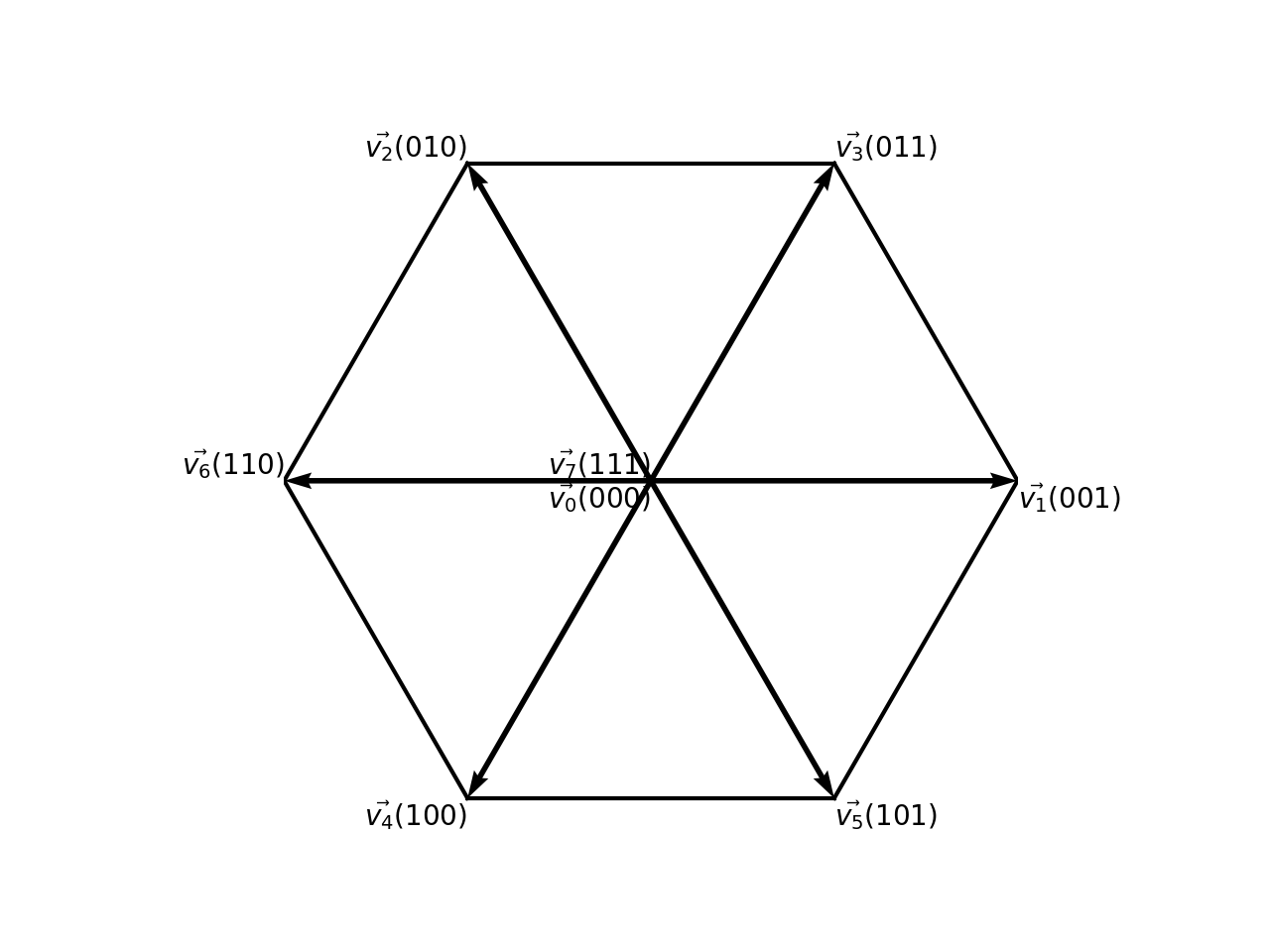
If we draw lines that go from one vector edge to the other we can observe that these lines form an hexagon as shown below.

(Source code, png, hires.png, pdf)

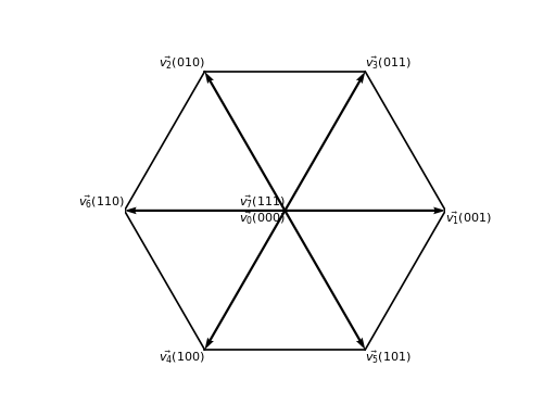
Fig. 6 SV-PWM synthesizable state vectors.

In order to synthesize an arbitrary voltage, there is a rather simple technique: given the sector in which the vector to be synthesized falls, we can quickly alternate between the two adjacent vectors. Taking a voltage falling in the first sector, i.e. \(\theta \in \left( 0, \frac{\pi}{3} \right)\), we have that the average space-vector \(\vec{v^a_s}\) is given by:

\[\left.\vec{v^a_s}\right|_{\text{sector} = 1} = \frac{1}{T} \left( x T \vec{v_1} + y T \vec{v_3} + z T \vec{0} \right) = x \vec{v_1} + y \vec{v_3}\]

where \(T\) is the averaging period and \(x + y + z = 1\). Note that \(z\) is the fraction of time where the actual voltage is zero (this happens for \(\vec{v_0}\) and \(\vec{v_7}\)). Replacing with values from Table 2 we have:

\[\hat{V_s} e^{j \theta_s} = x V_d e^{j 0} + y V_d e^{j \frac{\pi}{3}}\]

and by equaling both real and imaginary components, we obtain:

\[\begin{split}x &= \frac{\hat{V_s}}{V_d} \left( \cos(\theta_s) - \frac{1}{\sqrt{3}} \sin(\theta_s) \right) \\ y &= \frac{\hat{V_s}}{V_d} \frac{2}{\sqrt{3}} \sin(\theta_s).\end{split}\]

In terms of the \(\alpha\) and \(\beta\) components, we have:

\[\begin{split}x &= \frac{1}{V_d} \left( \hat{v_{\alpha}} - \frac{1}{\sqrt{3}} \hat{v_{\beta}} \right) \\ y &= \frac{1}{V_d} \frac{2}{\sqrt{3}} \hat{v_{\beta}}.\end{split}\]

If we repeat the previous calculation for each sector we get similar results. If we take:

(1)\[\begin{split}a &= x \\ b &= y \\ c &= -(x + y)\end{split}\]

being \(x, y\) the values obtained for the first sector, we can express the other values as a function of \(a, b, c\).

Table 3 SV-PWM X-Y

Sector	\(x\)	\(y\)
1	a	b
2	-c	-a
3	b	c
4	-a	-b
5	c	a
6	-b	-c

Sector determination

As we have already seen, knowledge of the sector is essential to compute the \(x, y\) values. If we are given the space vector in cartesian form, that is, \(v_{\alpha}\) and \(v_{\beta}\), we can easily determine its angle by performing \(\arctan\left(\frac{v_{\beta}}{v_{\alpha}}\right)\) and hence the sector. However, \(\arctan\) is an expensive trigonometric computation. It turns out there is a faster way to determine the sector.

If we take a look at the plot of Eq. (1) for all sectors, we have that each sector has a unique combination of signs:

(Source code, png, hires.png, pdf)

Fig. 8 Eq. (1) signs.

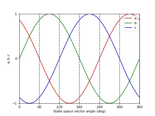
Sector	\(\text{sign}(a)\)	\(\text{sign}(b)\)	\(\text{sign}(c)\)
1	+	+	-
2	-	+	-
3	-	+	+
4	-	-	+
5	+	-	+
6	+	-	-

Amplitude limitation

By looking at the hexagon we can quickly observe that vectors falling in the middle of a sector will not have the same average amplitude as the ones that can be perfectly generated \(\vec{v_i}, i \in (0, ..., 7)\). The worst case happens for the space vectors falling just in the middle of the sector as shown on the figure below.

Fig. 10 Maximum synthesizable amplitude without distortion.

Therefore, in order to avoid distortions the maximum average amplitude should be limited to:

\[\hat{V_s}_{MAX} = V_d \cos(30^{\circ}) = V_d \frac{\sqrt{3}}{2}.\]

The previous value is actually the maximum line voltage we will be able to use when using SV-PWM.

Duty cycles calculation

Finally, we need to compute the PWM duty cycles using the values calculated in Table 3. When using a center-aligned PWM we have that the actual PWM output is “ON” when the control variable is over the trigger signal (a saw-tooth) and “OFF” otherwise.

There is still one thing left: the zero or null vector. Right at the beginning of this section we saw that in the formation of the space vector there is a fraction of time, \(z\), where a zero vector is active. There are actually a couple of zero vectors, \(\vec{v_0}\) and \(\vec{v_7}\). Both vectors are valid in order to produce the space vector, however, it is common to use the null-vector that only requires a single switch state change with respect to the previous or future state. This choice is also known as the reverse-alternating sequence. For example, if the next state is \(\vec{v_1}\) (001), then the null-vector choice would be \(\vec{v_0}\). Below the waveforms on the first sector are shown when using such sequence.

Fig. 11 PWM waveforms in sector 1 (\(z = z_0 + z_7\)).

By looking at the timing diagram in Fig. 11, we have that the duty cycles are for the first sector:

\[\begin{split}d_a &= x + y + \frac{z}{2} \\ d_b &= y + \frac{z}{2} \\ d_c &= \frac{z}{2}\end{split}\]

We can do a similar calculation for each sector, leading to the duty cycles listed in Table 4.

Table 4 SV-PWM duty cycle equations

Sector	\(d_a\)	\(d_b\)	\(d_c\)
1	\(x + y + \frac{z}{2}\)	\(y + \frac{z}{2}\)	\(\frac{z}{2}\)
2	\(x + \frac{z}{2}\)	\(x + y + \frac{z}{2}\)	\(\frac{z}{2}\)
3	\(\frac{z}{2}\)	\(x + y + \frac{z}{2}\)	\(y + \frac{z}{2}\)
4	\(\frac{z}{2}\)	\(x + \frac{z}{2}\)	\(x + y + \frac{z}{2}\)
5	\(y + \frac{z}{2}\)	\(\frac{z}{2}\)	\(x + y + \frac{z}{2}\)
6	\(x + y + \frac{z}{2}\)	\(\frac{z}{2}\)	\(x + \frac{z}{2}\)

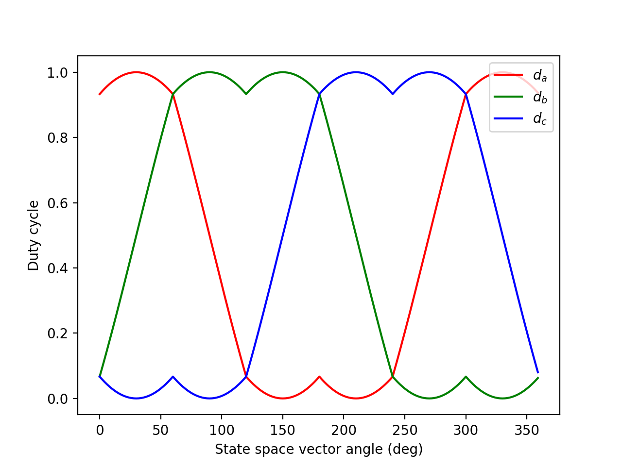
Using equations from Table 3 and Table 4 we can plot the duty cycle waveforms:

(Source code, png, hires.png, pdf)

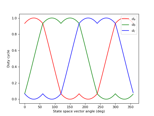
Fig. 12 SV-PWM duty cycle waveforms.